Evaluation of Impact of Statistical Tools on Process Performance Qualification (PPQ) Outcomes

This discussion paper uses segments of typical validation case studies (validation of key attributes such as: content uniformity, packaging key attributes and packaging critical defects) to apply various statistical tools and compare the outcomes of applying each tool pointing out the pros and cons of each application. General comment is also made on the statistical tools applied with some advantages, disadvantages and misuses briefly summarized.
Overview
In January 2011, the FDA issued a Guidance for Industry on “Process Validation: General Principles and Practices” [1]. In this guidance, process validation is defined “as the collection and evaluation of data, from the process design stage through commercial production, which establishes scientific evidence that a process is capable of consistently delivering quality product.” This paper examines numerous statistical analysis techniques for evaluating drug product performance data collected during Process Performance Qualification (i.e., Element 2 of the Process Qualification Stage). This paper also provides some general comments on the advantages and disadvantages of these statistical techniques.
1 Background and Scope
The 2011 FDA Process Validation guidance “outlines the general principles and approaches that FDA considers appropriate elements of process validation” and “aligns process validation activities with a product lifecycle concept and with existing FDA guidance, including the FDA/International Conference on Harmonization (ICH) Guidance for Industry, Q8 (R2) Pharmaceutical Development, Q9 Quality Risk Management, and Q10 Pharmaceutical Quality System.” The guidance states that “process validation involves a series of activities taking place over the lifecycle of the product and process” and that these activities are described in three stages, 1. Process Design, 2. Process Qualification, and 3. Continued Process Verification. The Process Qualification stage has two elements, 1. Facilities Design and Utilities and Equipment Qualification and 2. Process Performance Qualification (PPQ). This paper focuses on the evaluation of data collected during PPQ. The objective of PPQ is to collect and evaluate product performance data in order to demonstrate whether or not the process is in a state of control and to confirm whether or not the process is capable of producing batches that meet its quality requirements.
Justification of the sampling plan and acceptance criteria is required to be justified in the approved protocol; however, these elements are outside the scope of this paper.
There are multiple statistical analysis tools available to confirm whether or not the process is operating in a state control and/or confirm the product meets its quality requirements as measured via the output drug product quality. This paper presents some of the statistical tools which may be selected and the strengths and weaknesses of each.
2 Data Analysis and Review
This paper presents two data examples specifically uniformity of dosage and two packaging quality measurements. In each case, the data used for analysis were simulated to reflect data which may be expected from a typical manufacturing scenario.
2.1 Oral Solid Dosage Tablet Uniformity of Dosage Units (Content Uniformity)
Uniformity of dosage unit data was collected so that the drug content profile across each batch could be evaluated to determine if there are unexplained, unexpected, significant patterns in the attributes that could lead to bias or inaccurate interpretation of results during routine commercial distribution. Throughout the document the term Content Uniformity (CU) is used to describe the content of drug within the tablet by the Content Uniformity method.
2.1.1 Exploratory Data Analysis of Content Uniformity – Two Sampling Plans
Sampling Plan 1 represents a systematic random sample of 30 dosage units across the batch with one unit at the beginning, one unit at the end, and 28 equally spaced locations throughout the batch where the locations are not time based, but rather on the product volume. Sampling Plan 2 also represents a systematic random sample of 60 dosage units, with four units at the beginning, four units at the end, and four units at each of 13 equally spaced locations throughout the batch. The data used for Sample Plan 1 and Sample Plan 2 analysis are provided in Appendix 3 for reference. Table 15 provides a summary comparison of the impact of applying each of the statistical tools evaluated and Appendix 1 provides a general statistical summary of the tools.
Graphs are critical tools to any analytical analysis and should be the first analysis performed. They can provide insight into a data set regarding relationships and data integrity that a distilled statistic result, such as a mean or a p-value, cannot. This can be essential to the proper interpretation of the analysis. Conclusions regarding the significance of factors may be assessed with simple graphs followed by an appropriate analytical analysis, such as hypothesis testing or regression.
Sampling Plan 1
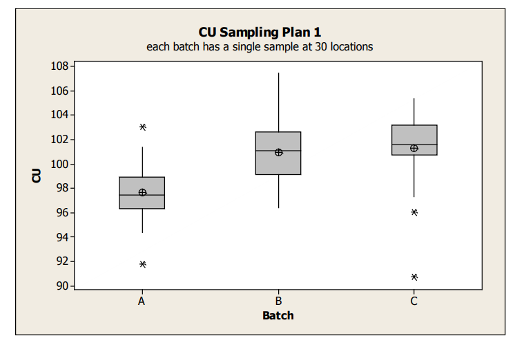
Boxplots display groups of data in their quartiles and can be used to display differences between populations without making assumptions of their statistical distribution. Box plots for the Sampling Plan 1 data is shown in Figure 1 and provide an overall sense of the distributions of data, including identification of potential outliers to a distribution. These outliers can represent real data or in some cases, are a quick indicator of data integrity issues. From this boxplot, it is clear that the average content uniformity result for Batch A tends to be lower than the other batches. This may be due to either special cause effects causing Batch A to be on average lower or random batch to batch variation. The within batch variation looks similar between the three batches.
figure 1 : Box Plots of Sampling Plan 1 Content Uniformity Data
Exploration can continue with individual value plots. These plots provide insight into the within batch variability not possible with the boxplots. For instance, Figures 2 and 3 illustrate two different ways to gain understanding about a potential location effect. Figure 2 uses a function in the software to identify the details associated with the selected data point(s), in this case, the location. Figure 3 shows the content uniformity results by location and are color coded by batch.
Figure 2: Individual Values Plots by Batch of Sampling Plan 1 Content Uniformity (CU) Data with ”brushing” tool to identify data features (location)
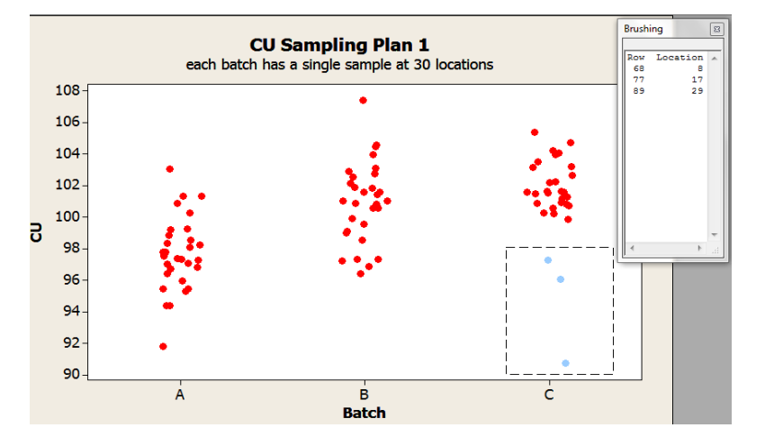
figure 3: Sampling Plan 1 CU Data Run- Chart by location with batch color code designation
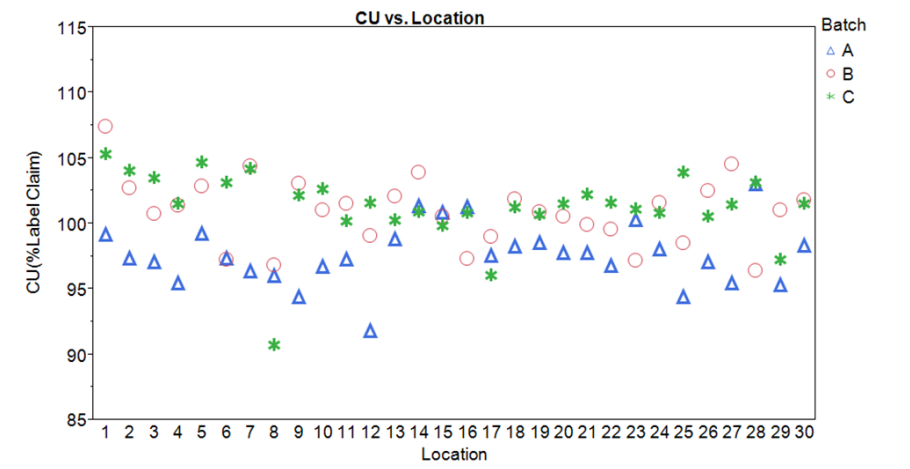
Note: the two highest results were drawn from location 1. The third result for that location was more typical. This could of course be random; it is impossible to draw any conclusions from this sample design. No other features related to location are evident.
Sampling Plan 2
Boxplots for the Sampling Plan 2 data is shown in Figure 4.
Figure 4: Sampling Plan 2 CU Data Box Plots by Batch
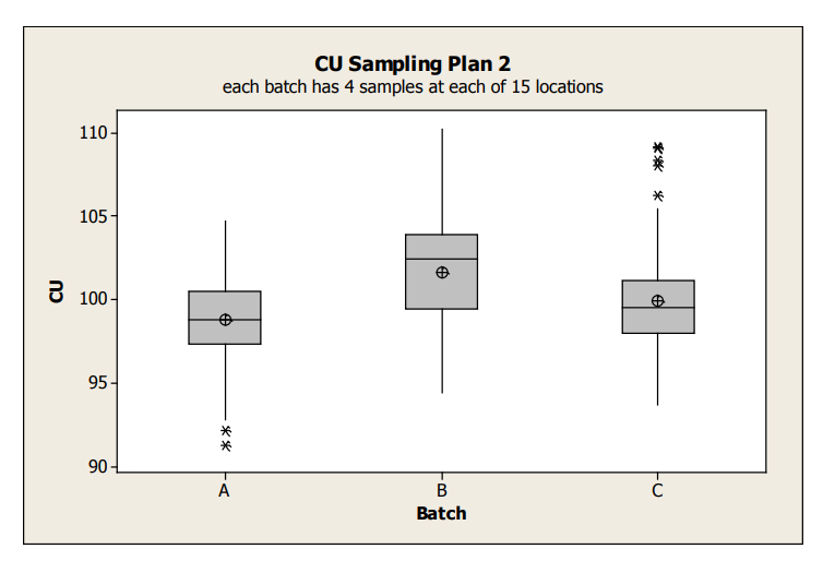
The average content uniformity for Batches A and C appear similar, while Batch B tends to be a bit greater. Note that this boxplot shows all variability within a batch; specifically since all of the data for each batch is combined, it does not allow visualizing whether the batch variation is due to between or within location. In order to understand these two different sources of variability, graphical exploration must go deeper. The following examples illustrate various graphical tools to better understand the variability between/within batches, and between/within location.
Figure 5: Sampling Plan 2 CU Line Plot by Location
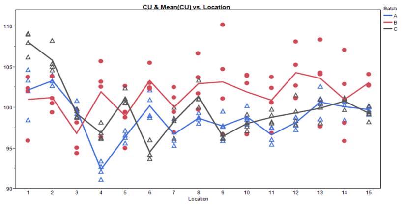
Figure 6: Sampling Plan 2 Batch by Location Scatter Plot
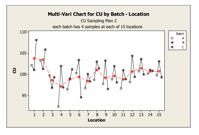
Figure 7: Sampling Plan 2 Location by Batch Scatter Plot
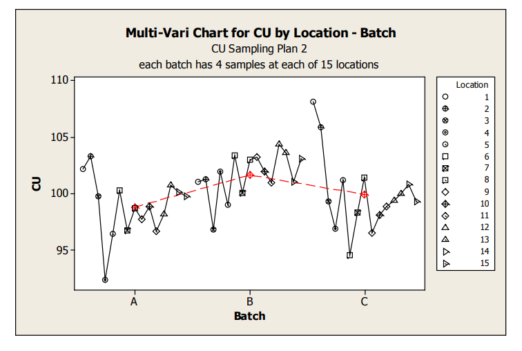
These graphs allow assessment of both location and batch effect not possible with the previous plots. Values for location 1 and 2 are relatively high for Batches A and C. A potential batch effect is also clear from this graph; Batch B has the highest value for all, but 4 locations (two of which are the abnormally high locations for Batches A and C) other than the low outlier for Batch A, locations 3 and 4 do not appear much lower compared to locations 5 to 15. The very low mean value observed for Batch A, location 4, is NOT due to a single outlying measurement; many measurements were low.
2.1.2 Variance Components
The manner in which samples are collected and tested can be structured to allow increased knowledge about the sources of variation. For example, several dosage units could be sampled from different locations in a batch (Sampling Plan 2) or several dosage units could be sampled from different batches. A more complicated structure might be multiple dosage units taken at different locations from multiple batches. Suppose that four dosage units are tested from 15 locations throughout a batch. The overall standard deviation of the 60 results could be calculated, but it ignores the structure of the data. To compare two test results, it might depend on whether the results came from the same location or different locations. There are two sources of variation: 1. within-location and 2. between-location. In the more complicated structure of Sampling Plan 2, the overall standard deviation would include within- location, between-location-within-batch, and batch-to-batch components of variation.
Variance component analysis is a statistical method to partition the overall variance into its individual components. This allows estimation of each component as well as a measure of the relative contribution of each component to the total variation. If the three batches of Sampling Plan 1 are combined, there are two variance components: 1. between-batch and 2. within-batch. For Sampling Plan 2 combining the three batches, there are three variance components: 1. between-batch, 2. between-location-within- batch, and 3. within-location. Point estimates and 95% confidence limits of the means and the variance components used in this document are presented in Tables 1 to 4. The means and variance components are used in the ASTM and Monte Carlo statistical methods presented in subsequent sections of the document.
| Batch | Point Estimate | 95% Confidence Limit | ||
|---|---|---|---|---|
| Mean | SD | Mean | SD | |
| A | 97.627 | 2.345 | 96.752 | 3.000 |
| B | 100.93 | 2.547 | 101.89 | 3.259 |
| C | 101.3 | 2.801 | 102.34 | 3.584 |
| Parameter | Point Estimate 95% | 95% Confidence Limit | |
|---|---|---|---|
| Overall Mean | 99.953 | 94.93 | |
| SD | Between-batch | 1.968*(p-value < 0.0001) | 8.918 |
| Within-batch | 2.571 | 2.941 | |
| Total | 3.237 | 9.391 | |
When the batches are combined in Sampling Plan 1, the between-batch SD confidence limit is very high, i.e., over four-fold the point estimate (Table 2, 8.918 vs. 1.968). This is due to the small number of batches tested (3). [The difference between the point and confidence interval estimates will decrease as the number of batches increases and is illustrated in Section 2.1.3.2, Figure 8.]
When the batches with nested location are combined in Sampling Plan 2 (Table 4), only the point estimates are used. This is because confidence limits for this more complicated variance structure are not practically meaningful again due to the limitation in number of batches.
Also, there is an assumption batches have similar within batch variability. This assumption was checked using the Bartlett Test and there was no significant difference between the within batch standard deviations (details not shown).
| Parameter | Batch A | Batch B | Batch C | ||||
|---|---|---|---|---|---|---|---|
| Point Estimate | 95% Confidence Limit | Point Estimate | 95% Confidence Limit | Point Estimate | 95% Confidence Limit | ||
| Mean | 98.8 | 97.3 | 101.6 | 102.7 | 99.9 | 98.0 | |
| SD | Between- location | 2.570* | 3.809 | 1.008** | 2.332 | 3.387 * | 4.979 |
| Within- location | 1.250 | 1.516 | 3.390 | 4.110 | 1.119 | 1.357 | |
| Total | 2.858 | 4.100 | 3.537 | 4.726 | 3.567 | 5.161 | |
* Significant (p-value < 0.0001) ** Not Significant (p-value = 0.21) | |||||||
| Parameter | Point Estimate |
|---|---|
| Overall Mean | 100.114 |
| Between-batch SD | 1.246*(p-value = 0.02) |
| Between-location[Batch] SD | 2.523*(p-value < 0.0001) |
| Within-location SD | 2.184 |
| Total | 3.562 |
| * Significant Variation | |
2.1.3 Monte Carlo Simulation
Monte Carlo simulation is used to estimate the probability of passing the USP content uniformity test. Monte Carlo simulation could be used in PPQ to determine the probability of passing for a given attribute and making decisions on the continuation or discontinuation of PPQ level sampling based on those projections. Computer-simulated data (100,000 batches) are generated from a normal distribution with mean and Standard Deviation (SD) estimated from the test data. The mean and standard deviation estimates are either on a point estimate basis or 95% confidence limit basis. Variance component analysis (see Section 2.1.2) is applied to the test data to estimate the between-batch and within-batch variances when batches are combined in Sampling Plan 1. Analysis of Sampling Plan 2 for each batch is similar, except location is designated as the factor. When the three batches are combined for Sampling Plan 2, then as noted above, the structure has three components, between-batch, between-location- within-batch, and within-location. This kind of structure is called nested since each batch has its own set of locations and each location has its own set of dosage units. The percentage of simulated batches passing the two-staged content uniformity test criteria is then determined.
2.1.3.1 Applying Monte Carlo Simulation to Evaluate the Probability of Passing the Harmonized Pharmacopeial Content Uniformity Test
2.1.3.1.1 Sample Plan 1 by Vatch
Batches A and B can be shown to be normally distributed; Batch C cannot, due to a slight left-skew (Figure 2). Before performing any data transformation to normalize a data distribution, investigation should first be conducted to explore why non-normality exists (e.g., analytical, process, data entry, etc.) Certain issues could cause tests of normality to fail (e.g., due to lack of precision in reporting significant figures, etc.), but from a practical perspective, the data can still be considered normally distributed. Further readings on treating non-normal data are given in the references.1 In this paper, Batch C is treated as approximately normal. Using the point estimate basis, all of the simulated batches pass content uniformity. Using the confidence limit basis, there is a small percentage that fails S1, but all pass the overall criteria. Simulating from Batch C, ignoring its slight deviation from normal distribution, may not accurately reflect the performance of its future batches.
| Batch | Point Estimate | Confidence Limit | ||
|---|---|---|---|---|
| S1 | S1 and S2 | S1 | S1 and S2 | |
| A | 100 | 100 | 99.9 | 100 |
| B | 100 | 100 | 99.9 | 100 |
| C | 100 | 100 | 99.2 | 100 |
2.1.3.2 Sampling Plan 1 – Combined Batch
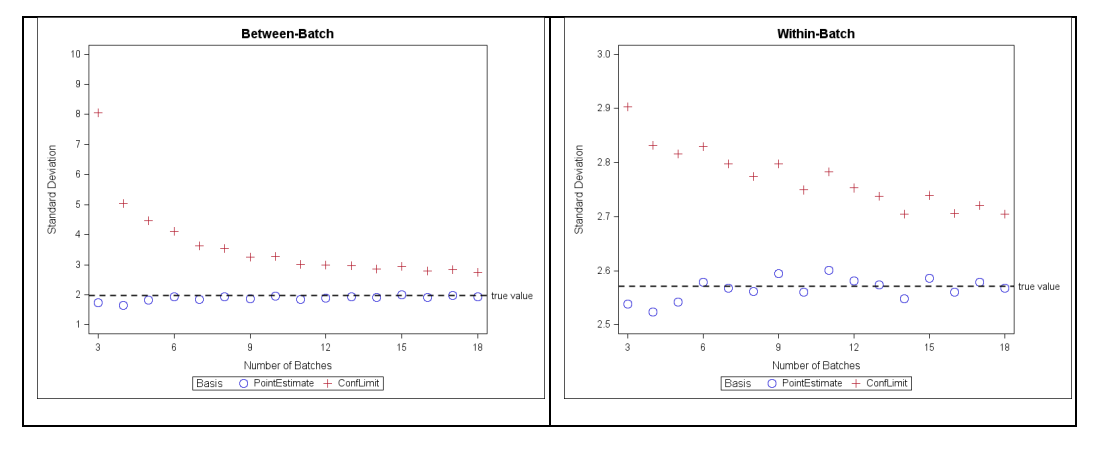
When the three batches are combined together, the between-batch SD point estimate is 1.968. There is 100% overall passing using point estimates. The between-batch SD confidence limit (8.918) is over four- fold the point estimate due to having only n=3 of batches. Consequently, there is only a 70% overall passing using the confidence limit basis (Table 6). When number of batches is increased, the confidence bound on SDs will be more precise so the corresponding percentage passing is expected to increase. As an illustration, the between- and within-batch SD estimates in Table 2 along with mean=100 are designated as “true” parameters of a process. A set of 100 simulations of increasing numbers of batches are drawn from this process and the point estimates and upper confidence bounds of the components of variance are calculated. The averaged results from the 100 simulation sets are plotted as a function of number of simulated batches (Figure 8). For this example, when number of batches is at least 10, the upper confidence bounds of between- and within-batch SDs more closely approximate the true parameters.
| Point Estimate | Confidence Limit | ||
|---|---|---|---|
| S1 | S1 and S2 | S1 | S1 and S2 |
| 100.0 | 100 | 64.3 | 70 |
Figure 8: Point estimate and upper confidence bound standard deviation vs. number of simulated batches for between-batch (left panel) and within-batch (right panel); simulation parameters: mean = 100, between-SD = 1.968, within-batch=2.571, 100 set-simulation
2.1.3.1 Sampling Plan 2 – By Batch
The first few location measurement in Batches A and C are shifted resulting in large location-to-location variability (point estimates of between-location SD are 2.570 and 3.387, respectively, Table 3). There is smaller location-to-location variability in Batch B (1.008). However, the variability within a location is large (3.390). There is 100% overall passing using point estimates. Using confidence bound basis, Batch B has the lowest percentage passing of 87.4% at S1 and 98.4% overall.
| Batch | Point Estimate | Confidence Limit | ||
|---|---|---|---|---|
| S1 | S1 and S2 | S1 | S1 and S2 | |
| A | 100 | 100 | 99.5 | 99.8 |
| B | 99.7 | 100 | 87.4 | 98.4 |
| C | 100 | 100 | 98.6 | 99.1 |
2.1.3.2 Sampling Plan 2 – Combined Batches
In this paper, the location is nested under batch (refer to description of a nested design in the section 2.1.2). When the three batches are combined, the total variance includes between-batch, between-
location [nested under batch], and within-location variances. Using the SD point estimates in simulation, there is a 100% overall pass rate. A confidence bound basis is not presented as it is not practically meaningful since there are only n=3 batches.
| Point Estimate | |
|---|---|
| S1 | S1 and S2 |
| 100.0 | 100.0 |
2.1.4 ASTM E2709 and E2810 (Historically also Referred to as CuDAL)
The two sets of content uniformity data generated by Sampling Plans 1 and 2 were evaluated using ASTM E2709/E2810. ASTM E2709 provides the general methodology whereas E2810 applies the methodology specifically to content uniformity data generated either by Sampling Plan 1 (one unit tested at each of several locations) or Sampling Plan 2 (more than one unit tested at each location). The methodology generates an acceptance limit table that if passed assures with a specified level of confidence (usually 90% or 95%) that there is at least a specified probability (called coverage, usual set at 95%) that a sample from that particular batch and tested against the USP Uniformity of Dosage Units
<905> will pass. The evaluation of each sampling plans data is given below:
Sampling Plan 1 Evaluation
The ASTM method for Sampling Plan 1 requires computing the mean and standard deviation of the 30 results which are shown in Table 9 in the variance component section. To pass the ASTM E2810 method requires that the computed standard deviation is less than a standard deviation listed in an acceptance limit table. The appropriate acceptance limit table depends on the desired confidence level, the coverage, and the sample size. The acceptance limit for n=30 and 95% coverage are given in table 9 for both the 90% and 95% confidence levels.
Table 9: Content Uniformity Sampling Plan 1 Acceptance Limit Table for N=30
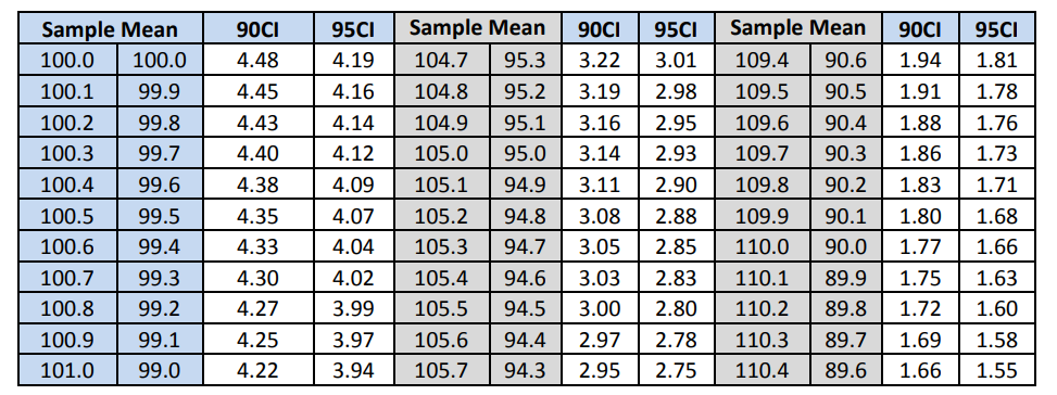
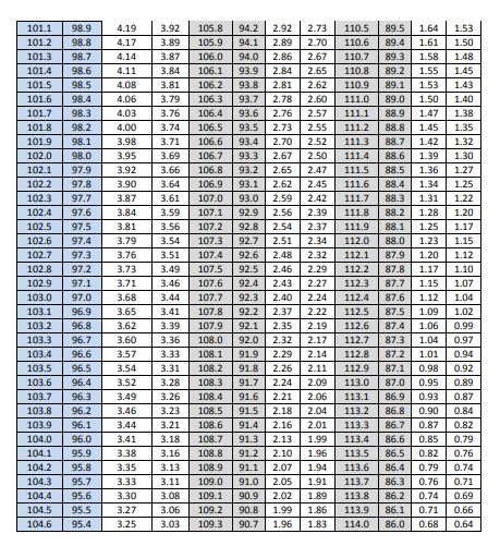
The acceptance limits corresponding to the computed means are given in Table 10 along with the decision as to whether or not the computed standard deviation pass the acceptance table limit. Note that all three batches pass the ASTM criteria.
| By Batch | |||
|---|---|---|---|
| ASTM E2810 | Batch | ||
| 90%CI/95% Cov | A | B | C |
| STD DEV Limit | 3.84 | 4.22 | 4.14 |
| Decision | Pass | Pass | Pass |
| 95%CI/95%Cov | |||
| STD DEV Limit | 3.20 | 3.52 | 3.45 |
| Decision | Pass | Pass | Pass |
As noted above, the ASTM method only applies to the batch tested. However, based on the available batches, there is a way to evaluate the probability that future batches will pass the ASTM method. This is done by simulation as discussed in Section 2.1.5. A Monte Carlo simulation was performed to estimate the probability of passing different ASTM acceptance limit tables. For sample sizes of 10, 20, 30, and 60 and confidence levels of 90% and 95% coverage, one hundred thousand sets of content uniformity results were generated and the number of times that the ASTM acceptance limit tables were passed was calculated. The simulation was performed, similar to Section 2.1.5.1.2, assuming that the ‘true’ between and within batch standard deviations were equal to the point estimates and then they were done again using the confidence limits on the overall all mean of the three batch as well as the upper 95% confidence limits on the between and within standard deviations. The results are given in Table 11.
| Across Batches | ||
|---|---|---|
| P(Batches Passing UDU or ASTM E2810) | Point Estimates 95% | Confidence Intervals |
| ASTM | ||
| 90%CI/95% Cov | ||
| N=10 | 69.51 | 16.93 |
| N=20 | 97.24 | 33.06 |
| N=30 | 99.58 | 40.02 |
| N=60 | 99.96 | 47.84 |
| 95%CI/95% Cov | ||
| N=10 | 49.25 | 9.65 |
| N=20 | 92.89 | 25.78 |
| N=30 | 98.79 | 34.87 |
| N=60 | 99.94 | 45.05 |
The simulation results can be very useful in selecting a sample size for future batches. For example, using the point estimates, there is only a 69.51% chance that samples of size 10 will pass the 90%CI/95% Coverage acceptance limit tables. But a sample of size 30 would have at least a 99.5% chance of passing. Notice that the probability of passing the tables based on the upper confidence intervals is very low.
This is due to the high estimate of the between batch standard deviation caused by only having three batches.
An assumption of combining batches is that the variances within batches are similar. Two tests which are used for testing this assumption are Bartlett’s and Levene, which in this case indicated similarity (individual batch standard deviations are 2.34%, 2.55%, 2.80%).
Sampling Plan 2 Evaluation
The ASTM method for Sampling Plan 2 requires calculating the overall batch mean, the standard deviation of location means, and the average within batch (pooled) standard deviation. To pass the ASTM E2810 method requires that the observed overall mean falls between two limits. The two limits on the mean depend on the observed standard deviation of location means (note that this is just the standard deviation of the location means – not the between location variance component) and the within location standard deviation. As for Sampling Plan 1, the appropriate acceptance limit table depends on the desired confidence level, the coverage, the number of locations, and the number of dosage units tested per location. The acceptance limit table for 15 locations with 4 dosage units per location is provided as Appendix 5. The acceptance limit range for the overall mean corresponding to the observed standard deviation of location means and within location standard deviation are given in Table 12 along with the decision as to whether or not the observed standard deviation passing the acceptance table limit. Note that all three batches pass the ASTM criteria using the 90% confidence level, but batch C does not pass the 95% confidence level. This is due to the high between location variability.
| By Batch | |||
|---|---|---|---|
ASTM E2810 | Batch | ||
| A | B | C | |
| Overall Mean | 98.80 | 101.64 | 99.90 |
| Between Location STD | 2.645 | 1.972 | 3.433 |
| Within Location STD | 1.250 | 3.390 | 1.119 |
| 90%CI/95% Cov Acceptance Table Range | 95.8-104.2 | 95.9-104.1 | 99.2-100.8 |
| Decision | Pass | Pass | Pass |
| 95%CI/95% Cov Acceptance Table Range | 97.1-102.9 | 96.8-103.2 | * |
| Decision | Pass | Pass | Fail |
| *Not possible at this confidence and coverage level. | |||
As noted above, the ASTM method only applies to the batch tested. However, based on the available batches, there is a way to evaluate the probability that future batches will pass the ASTM method. This is done by simulation. As in Sampling Plan 1, variance components is a way to take all of the variability in the data collected across the batches and divide it into separate “components.” In the situation where there are content uniformity results from several locations within different batches, the total variability can be divided into between batch variability, between location within batch variability, and within
location variability. Table 4 shows the estimated standard deviations for the between-batch, between- location, and within-batch variability. Both the between-batch and between-location standard deviations of 1.246%Label Claim and 2.523%Label Claim are significant. The within-batch standard deviation is 2.184%Label Claim for a total standard deviation of 3.562% Label Claim. The 1.246, 2.523, 2.184, and 3.562% estimates are called point estimates since they are the best estimates of the “true” batch standard deviations.
A simulation was performed to estimate the probability of passing different ASTM acceptance limit tables. For sample sizes of 10, 20, 30, and 60 and confidence levels of 90 and 95%, one hundred thousand sets of content uniformity results were generated and the number of times that the ASTM acceptance limit tables were passed was calculated. The simulation was performed assuming that the ‘true’ between-batch, between-location, and within-batch standard deviations were equal to the point estimates. The results are given in Table 13.
| Across Batches | |
|---|---|
| Simulations | |
| P(Batches Passing ASTM E2810) | Using Point Estimates |
| ASTM | |
| 90%CI/95% Cov | |
| N=10 | 32.67% |
| N=20 | 73.71% |
| N=30 | 91.78% |
| N=60 | 99.37% |
| 95%CI/95% Cov | |
| N=10 | 17.88% |
| N=20 | 55.79% |
| N=30 | 81.98% |
| N=60 | 98.52% |
The simulation results can be very useful in selecting a sample size for future batches. For example, there is only a 32.67% chance that samples of size 10 will pass the 90%CI/95% Coverage acceptance limit tables. But a sample of size 60 would have at least a 99.3% chance of passing. Note that the total standard deviation is over 3.5%. There is also significant batch to batch and location to location variability. If either of these variances could be reduced, the probabilities in the simulation would increase.
2.1.5 Statistical Intervals
For the statistical intervals analysis, consistency of content (uniformity of dosage units) has been defined in terms of the minimum proportion of units within an upper and lower limit or a maximum allowable proportion of units outside those limits. As stated in Hahn and Meeker, a statistical tolerance interval when evaluated against pre-specified limits may be used to demonstrate whether or not a specified proportion of “sampled” population meets the required limits (inference to the proportion of untested units that lies in the center of the specifications) or whether or not the proportion of units outside the limits exceeds a specified proportion (inference to the proportion of untested units that lie outside the specifications). Sampled population in this does not mean just the units tested, but applies to the untested units. The statistical intervals were computed using a stated confidence level of 95%, a minimum coverage proportion of 87.5% within pre-specified limits, maximum proportion of 6.25% outside pre-specified limits, and the pre-specified limits of 85%LC and 115%LC. The selection of confidence, coverage and pre-specified limits used in this section of the document are not recommendations of the authors of this paper. They were selected to illustrate how statistical intervals could be used when assessing uniformity of dosage units. In addition, the selected confidence, coverage and pre-specified limits are discussed in context to USP UDU requirements in Shen and Tsong’s 2011 USP Stimuli Article Bias of the USP Harmonized Test for Dose Content Uniformity.
Three types of statistical intervals were computed:
- Parametric Two-sided Tolerance Interval (PTS-TI)
- Parametric Two One-sided Tolerance Interval (PTI-TOST)
- Upper Confidence Bound on True Proportion for a Binomial Population (UCB on Binomial Proportion)
The first two types of intervals are appropriate for use when the drug content should be and has been shown to be normally distributed and free of significant process and analytical trends. The third type of interval is based on the binomial distribution and should be used when the sampled population is deemed to be infinite in size (i.e., greater than 2000 units) and when no more than 10% of the population is sampled. The third interval type can be used no matter the underlying distribution of the sampled population since the characteristic of interest (in this case, tablet content) is judged to be within the specified limits or outside the pre-specified limits. As is true for all the statistical assessments used in this paper, the intervals are only as valid as the sampling (random and representative) and testing (acceptable accuracy and precision) procedures that are used to obtain the drug content results.
A summary of the results from the statistical interval analyses is provided below.
- For all three batches, the PTS-TI tolerance intervals were within 85% to 115%LC. Using the PTS- TI results strictly as pass/fail acceptance criteria, it can be concluded with 95% confidence that at least 87.5% of the tablets in each batch have drug content within 85% to 115 %LC. When using the PTS-TI results for obtaining a confidence interval on the population, it can be concluded with 95% confidence that at least 87.5% of the tablets in the sampled population have drug content within the TL ,TU . For example, the 95% PTS-TI for Batch 1 of Sampling Plan 1, it can be concluded with 95% confidence that at least 87.5% of the tablets have content between (92.9 %LC, 103.1 %LC).
- For all three batches, the PTI-TOST lower tolerance bounds were greater than 85 %LC and the upper tolerance bounds were less than 115 %LC. Using the PTI-TOST assessment strictly as pass/fail acceptance criteria, it can be concluded with 95% confidence that no more than 6.25% of the tablets in each batch have drug content below 85% and with 95% confidence that no more than 6.25% of the of the tablets in each batch have drug content above 115 %LC. When using the PTI-TOST results for obtaining a 95% one-sided lower tolerance bound and a 95% one- sided upper tolerance bound, it can be concluded with 95% confidence that at no more than 6.25% of the tablets in the sampled population have drug content below TL and it can be concluded with 95% confidence that at least no more than 6.25% of the tablets in the sampled population have drug content above TU . For example, the 95% PTI-TOST for Batch 1 of Sampling Plan 1, it can be concluded with 95% confidence that no more than 6.25% of the tablets have content below 92.7 %LC and no more than 6.25% of the tablets have content above 102.5 %LC.
- For each individual batch, the 95% upper confidence bound on the percent of tablets with drug content below 85 %LC is 9.5% and the 95% upper confidence bound on the percent of tablets with drug content above 115 %LC is 9.5%. As no underlying distribution is assumed and the samples are considered to be randomly selected units from three consecutive batches of the process under assessments the data may be pooled; the 95% upper confidence bound on the percent of tablets with drug content below 85 %LC is 3.3% and the 95% upper confidence bound on the percent of tablets with drug content above 115 %LC is 3.3%. The 95% upper confidence bounds based on sampling 30 units and observing no units with content below 85 %LC and no units with content above 115 %LC exceeds the required 6.25%. Based on binomial distribution theory, to have achieved a 95% upper confidence bound below 6.25% even when no units are observed below 85 %LC or above 115 %LC, a minimum of 47 units would have been required to test. Therefore, testing 30 units per batch is not sufficient to demonstrate with 95% confidence that the true percentage of units below 85% or above 115% does not exceed 6.25%, when modeled using a binomial sampling distribution.
Both the PTI-TOST and the UCB Proportion approaches can be used as acceptance criteria that to ensure that there is at least a 95% probability of failing the acceptance criteria if the true percentage of tablets with content below 85% or above 115% is greater than or equal to 6.25%. The PTS-TI approach does not allow for a straightforward and “direct” consumer protection statement to be declared. It has been indicated in various publications that the PTI-TOST approach is preferred over the PTS-TI as it provides a better control of the proportion of tablets with content below 85 %LC and above 115 %LC.
2.1.6 Bayesian Statistics
A Bayesian prediction interval seems similar to a parametric tolerance interval as each result in a statement regarding the likelihood that results will fall within, or will be covered by, a given range. However, the underlying computation, and hence use and interpretation, is fundamentally quite different. For instance, the normal tolerance intervals discussed thus far can only be used to draw conclusions about the performance of the batch(es) for which it was derived, and require an assumption of normality. In contrast, because the Bayesian solution provides a probabilistic statement, not a confidence statement as in frequentist methods that rely on sampling uncertainty of a repeated event, it can be used to predict future behaviour. Bayesian methods allow flexibility for underlying distributions, and do not require variance homogeneity or balanced data. Estimating paramaters and propagating the uncertainty of tehses estimates when making predictions, is achievable with little restriction. In this example, the non-normality, small sample size, and complex variance structure that inhibited prediction, or resulted in very conservative results using other methods, are not hindrances in a Bayesian approach.
In this example, a Bayesian approach was used for both sampling plans to estimate three probabilities: 1. the probability that the assay results of future batches will be within the range of 85-115%, 2. the probability of the three PPQ batches passing USP <905>, and 3. the probability of future batches passing USP <905>. In order to estimate these probabilities using a Bayesian approach, it requires the following (high level) steps: 1. fit a model to the data, 2. assume a normal prior distribution for mean and a gamma distribution for variance, 3. perform Markov Chain Monte Carlo simulation to obtain a posterior distribution of the parameters, including uncertainty. To estimate the probability related to assay range, two additional steps are required: 4. obtain a predictive distribution of assay, and 5.) assess the probability that the 0.025 and .975 percentiles of this distribution will be outside specification. Figure 9 is an example of a posterior distribution estimated for this exercise.
Figure 9: Example of a Posterior Distribution Estimated for this Exercise
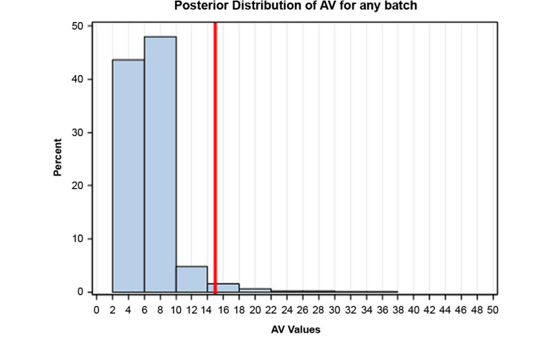
The Table lists the probability results for both Sampling Plan 1 and Sampling Plan 2.
| Sample Plan 1 | Sample Plan 2 | |
|---|---|---|
| Probability that 95% of future results will be within 85-115% | 89% | 96% |
| Probability that all three PPQ batches will pass USP<905> | 100% | 100% |
| Probability future results will pass USP<905> | 97% | 99% |
Note: the probability to pass USP<905> using a Bayesian approach is far higher than the value estimated using Monte Carlo simulation and a 95 %confidence bound for the parameters (97% vs. 64% listed in Table 6). Each method incorporates uncertainty into the prediction; however, use of a confidence bound is very conservative because it is highly influenced by the small sample size (three batches).
2.1.7 Capability
In general, process performance and process capability analyses are used to determine if the product from a manufacturing process is acceptable in respect to meeting product specifications. Performance and capability indices (PCIs) are derived from the output of process performance and capability analyses. Quite often, PCIs are computed without performing the necessary performance and capability analyses. Established consensus standards such as (ISO 22514 Parts 1 to 8 and ASTM E2281-08a) provide sufficient detail for correctly performing the process performance and process capability analyses.
The primary difference between capability and performance relates to statistical stability. Process capability is based on the inherent process variation (i.e., random cause variation) and process performance is based on the total process variation (i.e., both special cause and random cause variation). The voluntary consensus standard ISO/TR 22514-4:2007 differentiates process capability from process performance in that, process capability requires a process to have been demonstrated to be in a state of statistical control and the process to be controlled using a control chart. However, process performance does not require that the process be in a state of statistical control and does not require the process to be controlled using a control chart; in fact, retrospective data where the sequence of data is unknown can be used to evaluate process performance.
Process performance and process capability indices (PCIs) are used for determining the ability of a process to comply with specifications and they are used to estimate the percentage of results outside the specification limits. PCIs describe the tail behavior of the probability distribution of the characteristic of interest; therefore, the probability distribution (normal, non-normal, skewed, uniform, etc.) selected to model the process characteristic is essential for computing the PCIs. Process capability indices are denoted by (𝐶𝑝, 𝐶𝑝𝑘, 𝐶𝑝𝑘𝐿, 𝑎𝑛𝑑 𝐶𝑝𝑘𝑈) and process performance indices are denoted by
(𝑃𝑝, 𝑃𝑝𝑘, 𝑃𝑝𝑘𝐿, 𝑎𝑛𝑑 𝑃𝑝𝑘𝑈). The calculations of the PCIs are based on the ratio of the estimated process location and dispersion of the probability distribution selected to model the process and a reference specification interval.
Capability is generally calculated for responses that have specified upper and/or lower limits such as 90% to 110% label claim for potency. Since content uniformity does not have specific endpoints, a measure of capability might be determined by specifying a range of 85% to 115% label claim (e.g., the historical Stage 1 product expectations for content uniformity prior to Acceptance Value implementation).
Process capability is generally used for a process which requires a sufficient number of batches. As the means of the three processes are different and since there are only 3 batches available in the present data, a process capability would not be valid for this data. Although the criterion of a single mean is not required to estimate process performance, the small number of batches also makes the calculation of process performance inappropriate.
Prior batches may be used to calculate capability; however, the estimate of sigma (based on sample size) must be considered. The capability measure can still be determined for each batch to show that an individual batch is well within limits. For the reasons stated below, individual batch process capability estimates are not appropriate for Batch 3 for Sampling Plan 1.
Sampling Plan 1
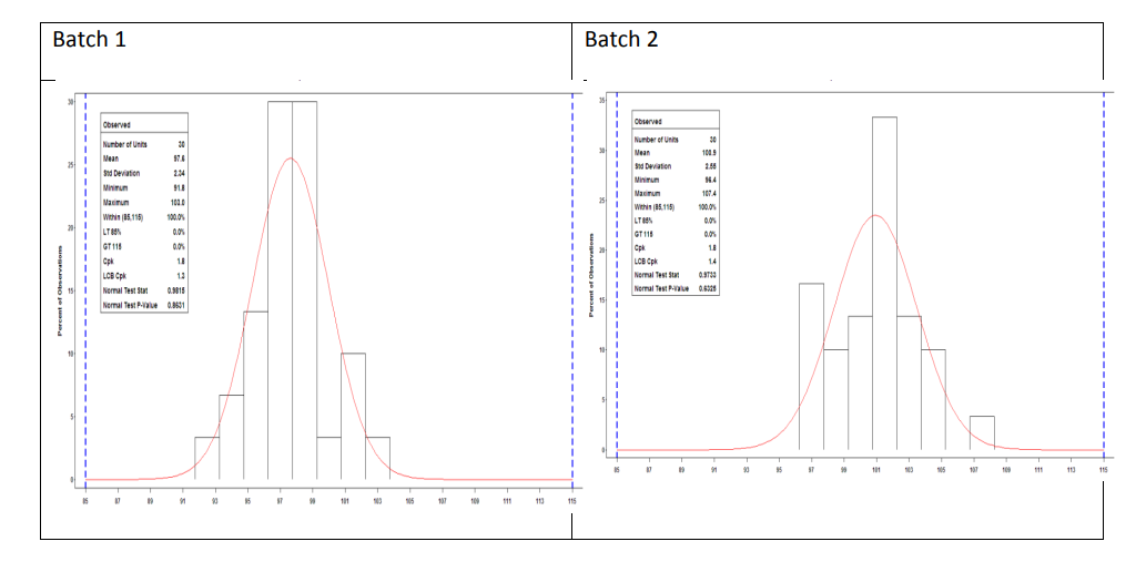
- Batch 1 is deemed to fit a normal distribution while demonstrating that it was manufactured in a state of statistical control.
- Batch 2 is deemed to fit a normal distribution while demonstrating that it was manufactured in a state of statistical control.
- Batch 3 is not deemed to fit a normal distribution and does not demonstrate that it was manufactured in a state of statistical control (see control chart section). Process performance for the batch could be calculated using the ISO standards but has not been calculated here.
The process capability estimate for Batch 1 and Batch 2 of Sampling Plan 1 is 1.8 with a 95% lower confidence bound of 1.3 and 1.4, respectively. This indicates that less than 0.01% of the tablet content results are outside 85 to 115% LC within each batch.
Capability for Sampling Plan 2 is more complex. It would not be appropriate to estimate a single simple standard deviation of all 180 data values. A more complex treatment of standard deviation such as found in ISO 22514 Parts 1, 2 and 4 must be applied. These calculations have not been included here.
Figure 10: Sampling Plan 1
2.1.8 Control Charts
Control charts may be used for evaluating process behaviour over time and are an excellent tool for identifying non-random variation within or across batches. Where a limited data set is available, typically fewer than 8 data points, time series plots may be used to provide a visual overview of process performance. Where larger data sets are available as in our data set for intra-batch performance, control charts may be used. For normally distributed data, typically control limits are established at approximately +/-3 Standard Deviations (SD) from the process mean; however, wider control limits (e.g., business driven limits) may be employed to provide a general view of the process performance where fewer data points are available for evaluation.
Control charts can provide information about the type and source of variation within a process. Variation may be classified in one of two ways as either common cause or special cause. Common cause variation is also called the natural pattern of the process and represents the routine, quantifiable variation in the process. Common cause variation exists in all processes, is fairly predictable, and is due to the combination of smaller sub-sets of variation which routinely exist within the process (e.g., equipment, people, test methods, materials, etc.) Special cause variation is unpredictable and is usually indicative of a identifiable event within the process (e.g., beginning of the process where segregation potential is higher for a powder mixture due to material fluidization during charging of the compression machine, drum or tote changes, humidity “hi-cups,” etc.) Special cause variation is typically easier to investigate, identify root cause and remediate that common cause variation issues (e.g., unacceptably large process variation or off target performance, etc.) For common cause variation, to achieve the level of desired process control, the inherent process variation must be reduced to an acceptable level.
In statistical process control, western electric rules are decision rules for detecting “out of control” or non-random conditions on control charts.2 Western electric rules are typically applied to statistical control charts to identify special cause variation. Western electric rules include data points outside of the statistical control limits, (e.g., nine) points in a row on either side of the process mean, (e.g., six) points in a row steadily increasing or decreasing and (e.g., 14 points) in row alternating up or down.(See ASTM 2587, ISO 7870-2 for specific values).
Statistical control limits should not be confused with specification limits. Statistical control limits are also often called the voice of the process and help determine if the process is “in-control” or if special cause variation exists. Statistical control limits may change as your process changes (e.g., raw material change, equipment change, etc.) Specification limits are the voice of the customer (patients) and typically would not change unless warranted by the patient. Typically, specifications are not included on control charts due to the potential to alter the data scale and interpretations.
For our Sample Plan 1 data (1 sample from 30 locations), I-MR control charts were used to analyze the intra and inter-batch performance. I-MR control charts are used when 1 result per analysis point is available. I-MR charts do not provide data of the within location variability of a process (e.g., if you were to sample location 1 repeatedly) but provide a good estimate of overall location to location performance.
As can be seen in Figure 11, when each batch (IMR) is graphically presented next to one another a good visual of inter-batch performance is also provided. From this IMR chart, we can see that the mean for Batch A (97.6%) was slightly lower than the mean for Batch B (100.9%) and C (101.3%) which were relatively closer to one another. Also, no significant differences were noted for the between batch variability, evidenced by the control limits and moving range values.
The moving range chart should always be evaluated first as this is a reflection of the amount of variation in the process. Moving range charts are used to detect changes in variation. If the range (R) chart indicates instability (e.g., numerous out of control limit points on the range chart), the individual values may lead one to believe an out of control process is in control.
Figure 11: Sample Plan 1, I-MR Charts of Three Batches
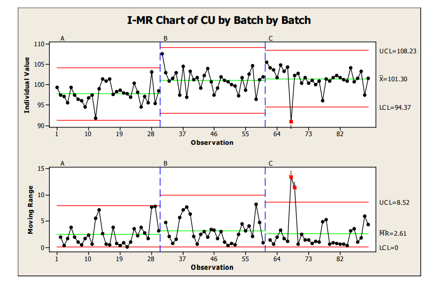
The control charts indicate within Batches A and B the process was in a state of statistical control. Batch C contained 1 data point (location 8 for the batch) from the Individual value chart (plot of individual measurements and the statistical control limits calculated for each of the individual batches) with an out of statistical control value. The moving range (range of 2 adjacent measurements) for this point and the next were also out of statistical control limits. An investigation would likely be conducted for Location 8 of Batch 3 to see if the result obtained for that location may be due to special cause variation (material handling, test occurrence, etc.) Location 12 from the first batch was within control limits, but also lower than the other results obtained for the batches. The proximity of Location 8 and 12 could be further evaluated to determine the root cause of the variation seen around this approximate location within the batch (e.g., tote change, or other event which may cause lower content uniformity, etc.) The low data points in this approximate location of the batch may warrant further study of the intra-batch performance to ensure with increased variability from other common cause variation that the process still performs robustly to the customer requirements. The degree of investigation taken will typically vary based on the degree of concern the results pose for indicating the process is out of control and/or the safety margin from the results versus the specifications.
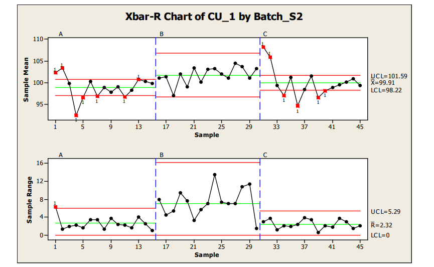
Analysis of Sample Plan 2, where 15 locations were sampled with 4 samples per location, is provided below via the use of Xbar-R (note: use of R vs S selection is samples per location dependent) control charts. As can be seen in the graphics, statistically out of control results were obtained for the sample range chart in Batch A and the sample means charts of both Batch A and C.
In sample range charts for Batch A and C, similar within location variability which was within control limits was seen. Batch B also contained data within the sample range control charts for all locations; however, wider within location variability was seen for Batch B. From the control charts, the mean and variation observed in Batch A and C appear to be relatively comparable. Batch A and especially C show a generally high start for the process; however, this statistical trend is not seen in Batch B, which tends to have a higher value and larger variation, resulting in the widest control limits for this batch.
The high starting point of Batches A and C and generally low behavior seen around locations 4 (Batch A) and 4 and 6 (Batch C) may be investigated for special cause variation sources. For all cases, the statistical control limits are well within values which would deliver passing acceptance value release limits. The statistical signals provide potential focus areas for enhancing the robustness of the process with the manufacture of future batches (reducing locational variation, improving process capability, etc.)
Figure 12: Sample Plan 2, X-R Chart of Three Batches Content Uniformity
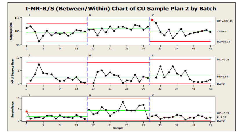
Another option for control charting is shown in Figure 13, an I-MR-R/S or Between/Within Chart. This chart is useful when the between location variability is not consistent with the within location variability. The individual points in the top chart are equivalent to the values in the X-bar chart. However, the control limits for these points are based on between location variability, instead of within location variability as in the X-bar-R/S. Because between-location variability is greater than within-location variability, the limits are wider.
Figure 13 : Sample Plan 2, IMR-R/S for Three Batches
2.1.9 Analysis of Variance (ANOVA)
Analysis of Variance (ANOVA) is a statistical method to compare treatment (e.g., batch) means of two or more treatments, or evaluate the variance component from nested effects. The computation and interpretation depends on the designation of the effects as “fixed” or “random.” A discussion of this distinction is not provided here; however, the authors recommend careful consideration of this distinction before applying ANOVA techniques. If the treatments are considered fixed and the goal is to compare all possible pairs of batch means, there are different tests developed to perform paired comparisons. One popular method is the Tukey-Kramer method which was used for the Sampling Plan 1 data in this document. The ANOVA results are provided in Table 15. The ANOVA table p-value of <0.0001 indicates that the three batch means are not equal to one another since the p-value is less than 0.05. The root mean square of 2.57% is the estimate of the within batch standard deviation. Result of the Tukey-Kramer test using an experiment-wise error of 0.05 (This means that there is a 5% chance of finding a significant difference between any pair of means if in fact the “true” batch means are the same) is shown by ordering the batch means from highest to lowest and then indicating which means are significantly different using different symbols. Any treatment means with the same symbol are not significantly different from one another. In this case, so Batches C and B are not significantly different from one another, but are both significantly different from Batch A. Note, that statistical significance must always be interpreted in context of practical difference and the statistical power of the test (not discussed here).
| Analysis of Variance | ||||
|---|---|---|---|---|
| Source | DF | Mean Square | F Ratio | Prob > F |
| Batch | 2 | 122.742 | 18.571 | <.0001* |
| Error | 87 | 6.609 | ||
| C. Total | 89 |
Root Mean Square Error = 2.57%LC
Connecting Letters Report (All Pairs Tukey-Kramer 0.05)
| Batch | Mean | |
|---|---|---|
| C | ● | 101.30 |
| B | ● | 100.93 |
| A | □ | 97.63 |
Levels not connected by same symbol (● or □) are significantly different.
| Statistical Method | Sample Plan | Key Findings from Data Set | Pass/Fail Applied Criteria |
|---|---|---|---|
| Graphical Exploration | Sample Plan 1- Per Batch Box Plot | Batch A lower average or batch to batch variability Within batch variation appears similar. | Not Applicable. |
| Sample Plan 1 - Per Batch Box Plot with Brushing | Batch A lower average or batch to batch variability. Within batch variation appears similar. Identification of location of outliers (Batch C Locs 8, 17 and 29) | ||
| Sample Plan 1 - Individual Values Plot Per Batch. | Two highest results drawn from Loc 1 (3rd result for location typical). | ||
| Sample Plan 2 Per Batch Box Plot | Averages for A & C appear similar. Batch B higher. | ||
| Sample Plan 2 - Individual and Location Mean Plot | Batch C higher at start than A & B. Batch A lower at location 4 than B and C. Higher individual values for Batch B including and beyond location 4. | ||
| Graphical Exploration | Sample Plan 2 - Multi-var by Batch Location Location | 1 and 2 relative high for Batch A and C with Batch C being very much higher relative to A and B. Batch B has the highest values for all, but 4 locs (with 2 abnormally high Statistical Method Sample Plan Key Findings from Data Set Pass/Fail Applied Criteria and Batch locations within Batch C). One outlier location for Batch A (low).
| |
| Variance Components | Sample Plan 1 | Significant Between batch variability. Between batch confidence interval is very high (due to low n large penalty paid). No significant difference between within batch SDs. | Not Applicable |
| Sample Plan 2 | Significant between batch and between location within batch variability | ||
| Monte Carlo Simulation | Sampling Plan 1 (By Batch) | The percentage of batches passing Stage 1 (S1) and overall S1 and Stage 2 (S2) of UDU is 100% based on point estimate basis. A small percentage (0.1-0.8%) fails S1, but still passes 100% the overall S1 & S2 using confidence interval basis. | Not Applicable Unless Pre-specified Criteria Established (e.g., 90%, 95%, etc. future passing) |
Sampling Plan 1 (Combined Batch) | The percentage of batches passing S1 and overall S1 & S2 is 100% based on point estimate basis. Only 64.3% of batches pass S1 and 70% pass overall S1 and S2 using confidence interval basis. This is due to having only three reference batches so the confidence intervals of variances are large. | Not Applicable Unless Pre-specified Criteria Established (e.g., 90%, 95%, etc. future passing) | |
| Sampling Plan 2 (By Batch) | Using point estimate basis, a small percentage (0.3%) fails S1 using batch B as reference batch due to high within-location variability; it still pass 100% overall S1 & S2 as do the other reference batches. Depending on the magnitude of between- and within-batch variances of reference batches, 87.4-99.5% pass S1 while 99.1-99.8% still pass overall S1 and S2 based in confidence interval basis. | Not Applicable Unless Pre-specified Criteria Established (e.g., 90%, 95%, etc. future passing) | |
| Sampling Plan 2 (Combined Batch) | The percentage of batches passing S1 and overall S1 and S2 is 100% based on point estimate basis. The confidence interval basis was not simulated due to more complex nested structure and the limited number of reference batches. | Not applicable | |
| Control Charts | Sample Plan 1 | Batch A and B in a state of statistical control. Western electric rule violations for Batch C. Batch C contained 1 out of control location (loc 8), indicating special cause variation may have occurred at this time point. Location 12 from Batch A was within control limits, but also lower than typical results and within relatively close proximity to Location 8. All batch means are similar. | Not applicable |
| Control Charts | Sample Plan 2 | Batch B in a state of statistical control. Western electric rule violations for Batches A and C. Higher within location variability was seen for Batch B. All batch means are similar. Location 1 and 2 are higher for Batches A and B, indicating a potential for special cause variation at the start of the batch locations. | Not applicable |
| ANOVA | “Fixed Batch | Batch B and C means are similar. Batch A mean is lower than Batch B and C mean | Not Applicable Unless Pre-Specified Criteria Established |
| ANOVA | “Random Batch” | Within batch variability contributes 63% of total variance. | Not Applicable Unless Pre-specified Criteria Established |
| ASTM2709/A STM2810 | Sample Plan 1 | Found Standard Deviations Less than ASTM E2810 Acceptance Limit Table Limit for Both 90% and 95% Confidence Level | All Individual Batches Pass Criteria at 90% and 95% confidence levels. |
| ASTM2709/A STM2810 | Sample Plan 2 | Found Overall Mean Within ASTM Acceptance Limit Table Range for 90% and 95% Confidence Level with the exception of Batch C at the 95% Confidence Level | All three batches pass Criteria at 90% confidence level. Batch A & B Pass at the 90% confidence level. Batch C fails at 95% Confidence Level. |
PTS-TI Tolerance Intervals | Sample Plan 1 | Calculated tolerance interval per batch: TL ,TU k30 = 1.996 Batch 1 92.9, 103.1 Batch 2 95.8, 107.4 Batch 3 97.5, 105.8 | All three batches pass with 95% confidence and 87.5% coverage of the 85% to 115% LC. 95% confidence that the percentage of tablets outside the range of (85%, 115%) label claim (LC) is less than 12.5%. |
PTI-TOST Tolerance Intervals | Sample Plan 1 | Calculated tolerance interval per batch: TL ,TU k30 = 2.084 Batch 1 92.7, 102.5 Batch 2 95.6, 106.2 Batch 3 97.3, 105.9 | All three batches pass with 95% confidence and 87.5% coverage of the 85% to 115% LC limiting the percentages of tablets below 85% and above 115% LC are both less than 6.25% of the lot. |
95% Upper Confidence Bound on proportion pU where | Individual Batch n tested units=30 x observed ≤85%LC=0 x observed ≥115%LC =0 95% One-Sided UCB | Individual batch: Insufficient sample size to analyze. | |
pUL =proportion ≤85 %LC pUU =proportion ≥115 %LC | pUL =9.5% and pUU =9.5% Due to low sample size (n=30) tool cannot demonstrate that the percentage of units below 85% is less than 6.25% or above 115% is less than 6.25% | ||
| Bayesian | Sample Plan 1 | There is 89% probability that 95% of results from future batches will have assay between 85-115% There is 97% probability that results will pass USP 905. | Not Applicable Unless Pre-specified Criteria Established (e.g. 90%, 95%, etc future passing) |
| Bayesian | Sample Plan 2 | There is 96% probability that 95% of results from future batches will have assay between 85 to 115% There is 99% probability that results will pass USP 905. | Not Applicable Unless Pre-specified Criteria Established (e.g., 90%, 95%, etc. future passing) |
| Process Capability Indices | Sample Plan 1 | Cpk of 1.8 with a 95% lower confidence bound of 1.3 and 1.4 Less than 0.01% of the tablet content results are outside 85 to 115% LC within each batch | Intra-batch determinations only made (due to low n=3) with low possible defect rate. Not Applicable Unless Pre-specified Criteria Established (e.g. Cpk > 1 with 95% confidence interval). |
| Process Capability Indices | Sample Plan 2 | Intra batch capability of 1.3 found with a 95% lower confidence bound of 1.0. This indicates that approximately 0.3% of the tablet content results could be outside 85 to 115% LC. | Intra-batch determinations only made (due to low n=3) with low possible defect rate. Not Applicable Unless Pre-specified Criteria Established (e.g. Cpk > 1 with 95% confidence interval). |
2.1.10 Packaging Quality Measurements (Fill Volume, Torque, Labeling, etc.)
The statistical methods used to evaluate measurements of packaging quality are often quite different than those used to assess process behavior. In many cases, packaging measurements are classified as attribute data (such as pass/fail), which require different methods than those used for continuous variables. In any case, the necessary conclusions from PPQ are the same: manufacturers must be able to show using statistical evidence that the process can consistently meet specification.
Acceptance sampling methods using ANSI standards Z1.4 and Z1.9 are often chosen to determine sample size for packing attributes. It is imperative that the user understand the assumptions, rules and statistical statements and risks associated with these methods. These methods are often misinterpreted as a means to draw conclusions regarding lot quality, during PPQ, and also during the commercial supply phase.
The following hypothetical examples explore statistical options, including the use of ANSI standards to evaluate process capability for common packaging measurements.
2.1.11 Bottle Fill Volume Example
In the first example, the packaging measurement is fill volume. Assume the following PPQ scenario for a liquid product, packaged in bottles:
- Packaging run time = 170 minutes
- Fill rate = 180 bottles/minute
- Total bottles filled = 30,600
- Filler has 6 nozzle heads
- Fill Volume Specifications: LSL = 99.5; USL = 100.5 ml
- AQL (acceptance quality limit) = 0.1%
(Note that the evaluation of fill volume described below would be applicable to other packaging measurements that are considered continuous variables, such as force measurements, like torque.)
There are multiple methods that are used to evaluate the acceptability of a filling process, including: 1. Acceptance sampling using ANSI Z1.9, 2. Control Charts and Process Capability, and 3. Acceptance sampling using ANZI Z1.4 (following conversion of continuous data to attribute data).
Assumptions for this hypothetical scenario:
- Process was stable with a mean and standard deviation of 100.2 and 0.08 ml respectively, for the first 26,000 bottles filled. For the remaining bottles, assume that one or two nozzles injected slightly more product, resulting in a “shifted” population having a mean of 100.35 and standard deviation of 0.09 ml.
- Samples from each nozzle were drawn at equally spaced intervals across the run.
2.1.11.1 Method 1: ANSI Z1.9
For a lot size of 30,600, an AQL of 0.1%, Variability Unknown, Double Specification, and a Tightened, Level II Inspection Criterion, a sample size of 100 is found from tables A-2 & B-3 of ANSI standard.
Because there are 6 nozzles, assume that 17 samples of 6 (total of 102) were drawn equally spaced across the run, specifically every 10 minutes.
To simulate possible outcomes for this hypothetical packaging situation, 14 samples of 6 were drawn from the initial population (mean = 100.2, standard deviation 0.08). The remaining three samples of 6 were drawn from the “shifted” population (mean = 100.35, standard deviation 0.09). This simulated draw of 17 samples of 6 resulted in a data set with the following characteristics:
Mean = 100.21
Standard deviation = 0.0907
Using the method defined by ANSI Z1.9, the following steps would be performed: Quality Index (upper) = (USL – mean)/s = (100.5– 100.21)/0.0907= 3.20
Quality Index (lower) = (mean – LSL)/s = (100.21– 99.5)/0.0907= 7.83
Estimate of Percent Ncf (non-conforming) above USL = 0.052 (Table B-5 of ANSI standard) Estimate of Percent Ncf below LSL = 0.00 (Table B-5 of ANSI standard)
Total Estimate of Percent Ncf = 0.052
Maximum Allowable Percent Ncf: 0.218 (Table B-3 of standard)
Conclusion: given the total estimate of percent Ncf is less than maximum allowable, the lot is accepted
Note that this conclusion is only valid as part of an ongoing acceptance sampling scheme; it is not to be interpreted as a lot quality statement. Acceptance sampling plans are designed to protect the producer from rejecting a lot that has a percent defective less than the AQL. The risk of missing a defective piece is not considered, and lots will be passed with an actual percent defective greater than the AQL, sometimes much greater. In order to manage both risks, the AQL should be balanced with the rejectable quality limit (RQL or lot tolerance percent defective LTPD) using the Operating Characteristic (OC) curve of the sampling plan. In this example, the actual percent nonconforming (bottles filled outside the range of 99.5-100.5 ml) for the simulated total lot of 30,600 bottles is 0.14%, which is higher than the AQL of 0.1%. Based on the Operating Characteristic Curve for this particular case, a sample size of 100 will result in lot acceptance 75% of the time; only 25% of the time will a bottle be randomly chosen that is out of specification. To control this risk and use the 0.1% specification as a lot tolerance percent defective, or rejectable quality limit, would require more samples. Only then could a claim regarding individual lot quality be made.
2.1.11.2 Method 2: Control Charts and Process Capability
The following X-bar/S group uses each time point of 6 samples as the subgroup. (Note: the use of an X- bar/S chart instead of an X-bar/R chart could be debated. Current thinking is that the S chart should be used for sample sizes much less than the typical minimum of 10.)
All statistical signals were applied to improve the likelihood of identification of a small shift in the mean.
Figure 14: X-R Chart of Samples
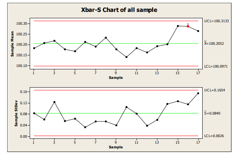
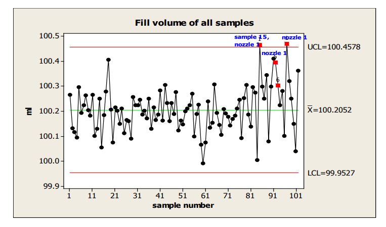
There is evidence of a shift at sample 15, flagged by Western Electric Rule 5, 2 of 3 consecutive measurements more than 2 sigma from the centerline.
In the next chart, an Individuals chart, which labels the nozzle used for the highest values, a potential nozzle effect is identified. (Note: the use of an I chart is not strictly correct, given the unlikelihood that nozzles within a sample would meet the independence requirement. However, it can be used in this situation to gain insight into the shift that is not provided by the X-bar/s chart.)
Figure 15: Individuals Chart with Identification of Nozzle with Highest Fill Volume
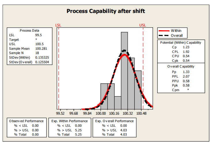
If this process behavior continues, a rough estimate of the % nonconforming based on the last 18 samples is about 4% and shown in the next capability plot.
Figure 16: Process Capability After Shift
2.1.11.3 Method 3: ANSI Z1.4
Sometimes packaging measurements of a continuous data type, such as fill volume and torque, are converted to a pass/fail measurement. The authors do not recommend this conversion routinely, as it leads to less available information and higher sample sizes. However, given this practice is not uncommon, and there are limited situations where this conversion is statistically warranted, an example is included here for comparison.
For a lot size of 30,600, an AQL of 0.1%, a Tightened, Level II Inspection Criterion, the required sample size is 800, with accept: reject of 1:2, based on Table II-B of ANSI standard Z1.4
In this hypothetical example that has an actual percent defective of 0.14%, this sampling scheme will result in acceptance of the lot 69% of the time. That is, there is only a 31% chance of rejecting the lot, even though the actual % defective is greater than the AQL. The likely acceptance of a lot that has a percent defective rate higher than the AQL results from the design of this approach, which is designed to have a high probability of acceptance up to the AQL (minimizes producer risk); it does not control the risk of not rejecting a batch with a percent defective greater than the RQL (consumer risk). In order to control the latter risk, a much greater sample size would be required. However, there are options such as double sampling plans that can potentially be applied to reduce the required number of samples, without increasing the sampling risk.
2.1.12 EXAMPLE 2 – Bottle Packaging Critical Defect such as an Incorrect Component
Assume the lot is 50,000 bottles, and the AQL is 0.065%
The same cautions discussed above regarding the use of acceptance sampling methods during PPQ to make statements of lot quality pertains to this example. Acceptance sampling methods are valid when applied to a continuum of lots as part of a sampling system. Unless the sampling is derived using an OC curve to provide a lot tolerance percent defective (LTPD or RQL), they do not provide a measurement of quality when applied to a limited number of batches, and therefore fall short of the requirements of PPQ.
2.1.12.1 Method 1
ANSI Z1.4 Tightened, Inspection Level II
Using Tables I and II-B of the standard, the required sample size is 1250, and the lot will be accepted if one or less nonconforming bottles are found. If the lot truly has a defective rate of 0.065%, there is only a 20% chance of rejecting the lot using this scheme.
2.1.12.2 Method 2
In the next method, an interval is estimated for the binomial proportion observed. There are multiple options for these estimates.3 One of these options, the Agresti and Coull interval, is found by adding two successes and two failures to the observed failure data, and estimating a 95% upper bound for the binomial proportion of the population.
Applied in this case of zero failures in 1250 samples, we can state with 95.0% confidence that the population nonconformance rate will be no more than 0.0050 (~.50%). This is much higher than the AQL of 0.065%. If the intent is to claim that the percent non-conforming is less than the AQL, many more samples would be required.
| Statistical Method | Example | Key Findings from Evaluation | Pass/Fail Applied Criteria |
|---|---|---|---|
ANSI Z1.9 Focus on AQL only | Fill Volume | Batch will pass criterion, with actual % non-conforming greater than the AQL. Batch having % non-conforming equal to the AQL will pass 75% of the time. | % non-conforming estimate for batch is 0.052; maximum % non-conforming according to standard to pass batch is 0.218. (which is greater than AQL). |
| Control Charts and Capability | Fill Volume | Shift in fill volume toward the end of the run. May be attributable to specific nozzle. | Rough estimate of Ppk, using limited data after shift is only 0.58. |
ANSI Z1.4 Focus on AQL only | Fill Volume | Batch will pass 69% of the time, even though actual % non-conforming is greater than the AQL. | 800 samples; accept: reject of 1:2. |
ANSI Z1.4 Focus on AQL only | Incorrect Component | Batch will be accepted 80% of the time if the non-conformance rate is as high as the AQL. | 1250 samples; accept: reject of 1:2. |
| Agresti & Coull Interval | Incorrect Component | If 0 non-conforming bottles are found in a sample of 1250, there is 95% confidence that the non-conformance rate will be no more than 0.5% | Acceptable non-conformance rate is 0.065%. |
Appendix 1 – General Comparison of Statistical Tools
Table A1: Comparison Table of Methods used in ISPE Case Studies
Clarify coverage definitions.
| Statistical Method | Statistical Statement that could be made | Advantages | Limitations--Applicable to what types of Data | Common Misuses Common Mistakes |
|---|---|---|---|---|
| Control Charts | Can distinguish between process variability that is likely from random, common causes (process in control), from that due to special, non-random causes (process out of control). Control limits bracket the expected variation of the process ( > 98% for mound shaped distributions, even when the distribution is heavily skewed). | Identify non-random features which indicate some relationship between the output and another factor. Can visually interpret the variability between batches and within batches (for replicate location sampling). Can provide a preliminary evaluation even for relatively small sample sizes using tentative control limits. | If sample size is too small, not a good estimate. The probability of occurrences for statistical signals depends on the underlying distribution. If the distribution is non- normal, the rate of false signals may be more than expected. (Level of inaccuracy depends on statistical signal and level of non-normality) Data set should include expected sources of variability. PPQ: Tools can be useful if multiple locations; not appropriate to go beyond these batches. Not linked to specifications. | Failure to recognize auto- correlation and its consequences. (e.g., the narrow control limits, statistical signals which are possibly expected). Choice of sample size based on finite number, not on sources of variability. Control limits are based on the analyzed data set which may inhibit identification of process changes within that data set Won’t look at cc until some finite number. Set the control limits to early – not including all sources of variability. Control chart selection for analysis (X-R/S or IMR/S, etc.). Misunderstanding between control limits and spec limits. Over reaction to statistical signals. Meant to guide further investigation and may not indicate quality concerns. |
| ANOVA | There is significant variation in group means (if locations are considered fixed) or significant variation among locations (if locations are considered random). | Statistical measure (p- value) of whether the observed difference (fixed) or location variability occurred by chance or is “real.”Easy to execute. | Assumptions: 1. Independence Factors outside of sampling plan that could affect the result are overlooked (e.g., API lot, laboratory precision factors) 2. Normality Data should be quantitative, not qualitative 3. Equal Variance Not linked to specifications. value. | Ending analysis with p-p-value significant: Treating as fixed, when in fact, it is random, and therefore, variance component should be estimated. Treating as random when it is fixed, and a location mean(s) comparison should be made. p-value insignificant: Interpretation of “no difference” to be equivalent to “equal” (no difference may be due to an insufficient number of locations. Could use OC curves. Number of locations should be designed prior to PPQ.) Making too many comparisons in fixed model (e.g., 20 pairwise comparisons). Not considering assumptions of ANOVA. |
| ANOVA “Random Location” | There is significant group to group variation. | |||
| ASTM 2709/ ASTM 2810 |
Passing the acceptance limit table for results obtained from a given sampling plan assures, with a pre-specified confidence level, that there is at least a pre- specified probability (called coverage) of passing the regulatory test (e.g., ICH harmonized UDU ) based on dosage units taken from that batch. | Method is tied directly to passing the regulatory test. Method incorporates uncertainty in the USP UDU conclusion due totablet to tablet and measurement variation. Can be used as a tool to meet the expectations set forth by FDA’s Process Validation Guidance (referenced in guidance). Easy to use Interpretation is desirable Allows user to provide their own levels of confidence and probability of passing regulatory test. Provides increased assurance with increased sample size Tied directly to regulatory requirements (Ensures compliance with 21 CFR 211.165(d)- testing and release for distribution). Can be used with significant between location variation. | Harder to pass than USP UDU test and may require larger sample sizes to achieve desired confidence/coverage. To use acce table for Sampling Plan 2 requires more calculations. To apply method to other regulatory tests other than dissolution or content uniformity (already done), mathematical derivations are required. If acceptance limit table does not exist for desired sampling plan, then a computer program is need to construct the limits. Company may want to use a different quality standard than passing the USP UDU test. ptance limit | Users extend the results from a single batch to all future batches. Method applies only to batch sampled – not to all future batchesSampled batch using Sampling Plan 2, but use acceptance limit table for Sampling Plan 1. Didn’t evaluate probability of passing acceptance limit table for selecting sample size resulting in too large or too small a sample size. |
| Monte Carlo Simulations | Probability of passing a method/procedure based on user provided inputs. | Provides a way of evaluating a method/procedure or process using computer generated data in place of collecting actual data. Flexible: User can develop their own model. | Small sample size (e.g., n=3) can provide poor estimates of the parameters and therefore unrealistically large confidence intervals which in turn result in low passing probabilities. * usefulness of method is only as good as reference data and the model; Complexity of use. | Using an inappropriate model (e.g., over simplified) Don’t generate enough data. Inaccuracy of result due to simulation error. |
| Tolerance Intervals | Assures with a pre- specified confidence level, that there is at least a pre-specified probability (called coverage) that the individual results will fall within the interval endpoints. | For Sampling Plan 1, easy to execute Allows for direct comparison to desired range (e.g., 85-115%) | Sampling Plan 2— interval is more complicated to generate. Sensitive to non- normality. |
Users extend the results from a single batch to all future batches. Method applies only to batch sampled – not to all future batches. Sampled batch using Sampling Plan 2, but use tolerance interval for Sampling Plan 1. Overlooking implication of small sample size, which may lead to wide intervals. |
| Bayesian Prediction Intervals | Provides the probability of the percentage of batches/units that will pass a specification. | Flexibility in underlying distribution assumptions (normality not required). Can apply to complex sampling plans. Can take advantage of prior information, no matter what the study design. | Requires Bayesian modeling and software expertise (various packages). | User choice of prior can affect results/conclusions (non-informative prior, etc.) |
| Process Capability Indices | Determines the ability of a process to comply with specifications. Also used to estimate the percentage of results outside the specification limits. | Directly linked to specifications and performance of process ability to meet specifications. Confidence interval may be applied on upper and lower bounds for enhanced understanding of performance. | Requires normally distributed data under statistical control for process capability (Cpk) determinations. Requires larger data sets (typically n> 20-30) for the most accurate estimations. Not sensitive to small process shifts. | Inappropriate grouping of varying sample sizes and/or data sets (e.g., different equipment or processes). |
| Variance Component | Estimated contribution of each source of variability and total variability | Provides ability to prioritize the sources of f variation for further focus if necessary to reduce total variation. Easy to execute. | Not linked to specifications | Overreaction to statistical significance without considering practical consequence (e.g., contribution of all sources is small relative to specification range) |
ANSI Z1.4 Acceptance Sampling for Attributes | The likelihood that a defective unit will be found, given a percent defective, is controlled by sampling plan. X% (chosen) probability the defect will be found if the true defect level is at or above the LTPD. | Access to sample tables. | No statistical statement regarding lot quality can be made. Basing the sample size on controlling the risk of acceptance of product below the AQL protects the producer, not the consumer. | Confusion regarding the alpha and beta risks of a sampling plan. Misinterpretation of AQL and RQL (LTPD). Disregard of operating characteristics curves to show the relationship between AQL & RQL. Sampling performed in an isolated format to make quality statements, instead of part of an ongoing acceptance plan with switching rules. |
ANSI Z1.9 Acceptance Sampling for Variables | Same as Z1.4 | Same as Z1.4 | Same as Z1.4 | The potential for information about the process gained from charts and capability analyses is overlooked. Same as Z1.4 |
Appendix 2 – Summary of Tolerance Interval Tools
| Method | Parametric Two-sided Tolerance Interval Plan PTS-TI | Parametric Two One-sided Tolerance Interval PTI-TOST | One-sided Upper Confidence Bound on True Proportion of a Population |
|---|---|---|---|
| Controls | Enclosure interval to contain or cover at least a specified proportion in the center of the distribution of a population with a specified confidence for a normal distribution. | Enclosure interval to ensure no more than a specified proportion in the tails of the distribution of a population with a specified confidence for a normal distribution. | Bound is on the actual percentage or proportion for binomial distribution. |
| Interval Parameter | (TL ,TU) (X - ks, X + ks) | (TL ,TU) =(X ks, X ks) | (pU ) |
| Interval Statistic | Tolerance factor k obtained by numerical iteration methods. | Tolerance factor k obtained by calculation using non-central t- distribution. | Upper confidence bound obtained using calculation based on F-distribution. |
| Published Journal/Book References | Hahn and Meeker 37(1) Stimuli to the Revision Process: Bias of the USP Harmonized Test for Dose Content Uniformity Meiyu Shen, PhD, Yi Tsong, PhD | Tsong, Yi and Shen, Meiyu (2007) 'Parametric Two-Stage Sequential Quality Assurance Test of Dose Content Uniformity', Journal of Biopharmaceutical Statistics, 17: 1, 143 — 157 D. B. Owen (1964) Control of Percentages in Both Tails of the Normal Distribution, Technometrics, 6:4, 377-387 Bias of the USP Harmonized Test for Dose Content Uniformity Meiyu Shen, PhD, Yi Tsong, PhD | C.J Clopper and E.S. Pearson (1934) ‘The Use of confidence or fiducial limits illustrated in the case of the binomial’, Biometrika 26, 404-413 Hahn and Meeker (H&M 1991 p103 to 104) |
| Voluntary Consensus Standard Reference | ISO 16269 -6 2005 ISO 2859-2 1985 E2762 – 10 | ISO 16269 -6 2005 | ISO 2859-2 1985 ASTM E1994 – 09 ASTM E141 – 10 ASTM E2334 – 2013 |
Appendix 3 – Sample Plan 1 Data Used in All Analysis
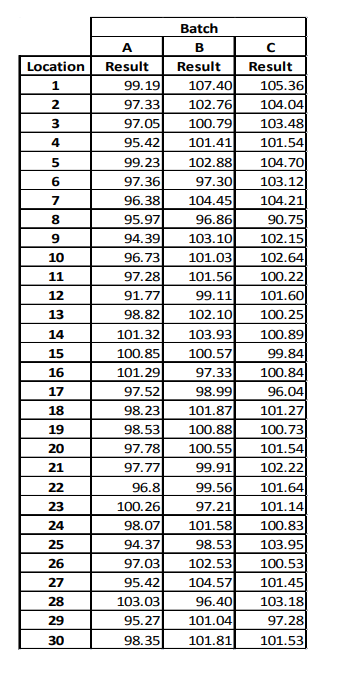
Appendix 4 – Sample Plan 2 Data Used in All Analyses
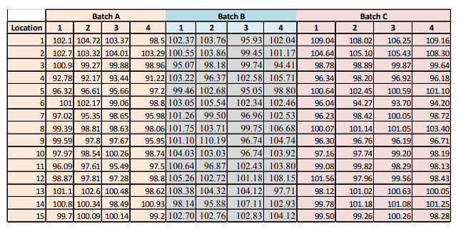
Limitations and Liability
In 2011, FDA issued a “Guidance for Industry Process Validation: General Principles and Practices Guidance”, which calls for a lifecycle approach to process validation and heavily references the use of statistics throughout the product lifecycle. For many, the use of statistics is new and could seem daunting due to the large number of possible statistical tools which could be used and the complexity of understanding the tools and ensuring they are appropriately applied. Statistics are a powerful tool which can enhance our level of process understanding and ultimately guide us to improve process performance and product quality/reliability.
This discussion paper uses segments of typical validation case studies (validation of key attributes such as: content uniformity, packaging key attributes and packaging critical defects) to apply various statistical tools and compare the outcomes of applying each tool pointing out the pros and cons of each application. General comment is also made on the statistical tools applied with some advantages, disadvantages and misuses briefly summarized.
This paper does not intend to teach or provide readers with a better understanding of the mathematics behind the tool, only to overview outcomes when applying each of the tools to the same data set.
Having this comparison may help guide selection of the most appropriate tool, or in most cases combination of tools, to inform the scientist validating the process of the level of process variation and control within and across batches. Readers are encouraged to work with trained statistical experts to ensure the tools are applied appropriately for their specific scenario taking into account the sample plan and intent of the analysis being conducted.
The team which worked on this paper hopes you find this exercise of value and appreciate your thoughts and suggestions to further the discussion on the topic of statistical analysis of validation data.
Please direct all feedback to pvpapers@ispe.org.
Acknowledgements
By Authors: Jim Bergum (Bergum STATS, LLC), Richard Montes (Hospira), Tara Scherder (Arlenda), Helen Strickland (GSK), Jenn Walsh (BMS)


